An Introduction to Management Science: Quantitative Approaches to Decision Making, Revised, 13th Edition solutions manual and test bank David R. Anderson | Dennis J. Sweeney | Thomas A. Williams | Jeffrey D. Camm | R. Kipp Martin
An Introduction to Linear Programming
Case Problem 1: Workload Balancing
1.
| Production Rate (minutes per printer) | |||
| Model | Line 1 | Line 2 | Profit Contribution ($) |
| DI-910 | 3 | 4 | 42 |
| DI-950 | 6 | 2 | 87 |
Capacity: 8 hours60 minutes/hour = 480 minutes per day
Let D1 = number of units of the DI-910 produced
D2 = number of units of the DI-950 produced
| Max | 42D1 | + | 87D2 | |||
| s.t. | ||||||
| 3D1 | + | 6D2 | £ | 480 | Line 1 Capacity | |
| 4D1 | + | 2D2 | £ | 480 | Line 2 Capacity |
D1, D2 ³ 0
The optimal solution is D1 = 0, D2 = 80. The value of the optimal solution is $6960.
Management would not implement this solution because no units of the DI-910 would be produced.
2. Adding the constraint D1 ³ D2 and resolving the linear program results in the optimal solution D1 = 53.333, D2 = 53.333. The value of the optimal solution is $6880.
3. Time spent on Line 1: 3(53.333) + 6(53.333) = 480 minutes
Time spent on Line 2: 4(53.333) + 2(53.333) = 320 minutes
Thus, the solution does not balance the total time spent on Line 1 and the total time spent on Line 2. This might be a concern to management if no other work assignments were available for the employees on Line 2.
4. Let T1 = total time spent on Line 1
T2 = total time spent on Line 2
Whatever the value of T2 is,
T1 £ T2 + 30
T1 ³ T2 - 30
Thus, with T1 = 3D1 + 6D2 and T2 = 4D1 + 2D2
3D1 + 6D2 £ 4D1 + 2D2 + 30
3D1 + 6D2 ³ 4D1 + 2D2 - 30
Hence,
-1D1 + 4D2 £ 30
-1D1 + 4D2 ³ -30
Rewriting the second constraint by multiplying both sides by -1, we obtain
-1D1 + 4D2 £ 30
1D1 - 4D2 £ 30
Adding these two constraints to the linear program formulated in part (2) and resolving we obtain the optimal solution D1 = 96.667, D2 = 31.667. The value of the optimal solution is $6815. Line 1 is scheduled for 480 minutes and Line 2 for 450 minutes. The effect of workload balancing is to reduce the total contribution to profit by $6880 - $6815 = $65 per shift.
5. The optimal solution is D1 = 106.667, D2 = 26.667. The total profit contribution is
42(106.667) + 87(26.667) = $6800
Comparing the solutions to part (4) and part (5), maximizing the number of printers produced (106.667 + 26.667 = 133.33) has increased the production by 133.33 - (96.667 + 31.667) = 5 printers but has reduced profit contribution by $6815 - $6800 = $15. But, this solution results in perfect workload balancing because the total time spent on each line is 480 minutes.
Case Problem 2: Production Strategy
1. Let BP100 = the number of BodyPlus 100 machines produced
BP200 = the number of BodyPlus 200 machines produced
| Max | 371BP100 | + | 461BP200 | |||
| s.t. | ||||||
| 8BP100 | + | 12BP200 | £ | 600 | Machining and Welding | |
| 5BP100 | + | 10BP200 | £ | 450 | Painting and Finishing | |
| 2BP100 | + | 2BP200 | £ | 140 | Assembly, Test, and Packaging | |
| -0.25BP100 | + | 0.75BP200 | ³ | 0 | BodyPlus 200 Requirement |
BP100, BP200 ³ 0
Optimal solution: BP100 = 50, BP200 = 50/3, profit = $26,233.33. Note: If the optimal solution is rounded to BP100 = 50, BP200 = 16.67, the value of the optimal solution will differ from the value shown. The value we show for the optimal solution is the same as the value that will be obtained if the problem is solved using a linear programming software package.
2. In the short run the requirement reduces profits. For instance, if the requirement were reduced to at least 24% of total production, the new optimal solution is BP100 = 1425/28, BP200 = 225/14, with a total profit of $26,290.18; thus, total profits would increase by $56.85. Note: If the optimal solution is rounded to BP100 = 50.89, BP200 = 16.07, the value of the optimal solution will differ from the value shown. The value we show for the optimal solution is the same as the value that will be obtained if the problem is solved using a linear programming software package such as Excel Solver.
3. If management really believes that the BodyPlus 200 can help position BFI as one of the leader's in high-end exercise equipment, the constraint requiring that the number of units of the BodyPlus 200 produced be at least 25% of total production should not be changed. Since the optimal solution uses all of the available machining and welding time, management should try to obtain additional hours of this resource.
Case Problem 3: Hart Venture Capital
1. Let S = fraction of the Security Systems project funded by HVC
M = fraction of the Market Analysis project funded by HVC
| Max | 1,800,000S | + | 1,600,000M | |||
| s.t. | ||||||
| 600,000S | + | 500,000M | £ | 800,000 | Year 1 | |
| 600,000S | + | 350,000M | £ | 700,000 | Year 2 | |
| 250,000S | + | 400,000M | £ | 500,000 | Year 3 | |
S | £ | 1 | Maximum for S | |||
M | £ | 1 | Maximum for M | |||
| S,M | ³ | 0 |
The solution obtained is shown below:
OPTIMAL SOLUTION
| 2486956.52174 | ||
| Variable | Value | Reduced Cost |
| S | 0.60870 | 0.00000 |
| M | 0.86957 | 0.00000 |
| Constraint | Slack/Surplus | Dual Value |
| 1 | 0.00000 | 2.78261 |
| 2 | 30434.78261 | 0.00000 |
| 3 | 0.00000 | 0.52174 |
| 4 | 0.39130 | 0.00000 |
| 5 | 0.13043 | 0.00000 |
| Objective | Allowable | Allowable |
| Coefficient | Increase | Decrease |
| 1800000.00000 | 120000.00000 | 800000.00000 |
| 1600000.00000 | 1280000.00000 | 100000.00000 |
| RHS | Allowable | Allowable |
| Value | Increase | Decrease |
| 800000.00000 | 22950.81967 | 60000.00000 |
| 700000.00000 | Infinite | 30434.78261 |
| 500000.00000 | 25000.00000 | 38888.88889 |
| 1.00000 | Infinite | 0.39130 |
| 1.00000 | Infinite | 0.13043 |
Thus, the optimal solution is S = 0.609 and M = 0.870. In other words, approximately 61% of the Security Systems project should be funded by HVC and 87% of the Market Analysis project should be funded by HVC.
The net present value of the investment is approximately $2,486,957.
2.
| Year 1 | Year 2 | Year 3 | |
| Security Systems | $365,400 | $365,400 | $152,250 |
| Market Analysis | $435,000 | $304,500 | $348,000 |
| Total | $800,400 | $669,900 | $500,250 |
Note: The totals for Year 1 and Year 3 are greater than the amounts available. The reason for this is that rounded values for the decision variables were used to compute the amount required in each year.
3. If up to $900,000 is available in year 1 we obtain a new optimal solution with S = 0.689 and M = 0.820. In other words, approximately 69% of the Security Systems project should be funded by HVC and 82% of the Market Analysis project should be funded by HVC.
The net present value of the investment is approximately $2,550,820.
The solution follows:
OPTIMAL SOLUTION
| Optimal Objective Value | ||
| 2550819.67213 | ||
| Variable | Value | Reduced Cost |
| S | 0.68852 | 0.00000 |
| M | 0.81967 | 0.00000 |
| Constraint | Slack/Surplus | Dual Value |
| 1 | 77049.18033 | 0.00000 |
| 2 | 0.00000 | 2.09836 |
| 3 | 0.00000 | 2.16393 |
| 4 | 0.31148 | 0.00000 |
| 5 | 0.18033 | 0.00000 |
| Objective | Allowable | Allowable |
| Coefficient | Increase | Decrease |
| 1800000.00000 | 942857.14286 | 800000.00000 |
| 1600000.00000 | 1280000.00000 | 550000.00000 |
| RHS | Allowable | Allowable |
| Value | Increase | Decrease |
| 900000.00000 | Infinite | 77049.18033 |
| 700000.00000 | 102173.91304 | 110000.00000 |
| 500000.00000 | 45833.33333 | 135714.28571 |
| 1.00000 | Infinite | 0.31148 |
| 1.00000 | Infinite | 0.18033 |
4. If an additional $100,000 is made available, the allocation plan would change as follows:
| Year 1 | Year 2 | Year 3 | |
| Security Systems | $413,400 | $413,400 | $172,250 |
| Market Analysis | $410,000 | $287,000 | $328,000 |
| Total | $823,400 | $700,400 | $500,250 |
5. Having additional funds available in year 1 will increase the total net present value. The value of the objective function increases from $2,486,957 to $2,550,820, a difference of $63,863. But, since the allocation plan shows that $823,400 is required in year 1, only $23,400 of the additional $100,00 is required. We can also determine this by looking at the slack variable for constraint 1 in the new solution. This value, 77049.180, shows that at the optimal solution approximately $77,049 of the $900,000 available is not used. Thus, the amount of funds required in year 1 is $900,000 - $77,049 = $822,951. In other words, only $22,951 of the additional $100,000 is required. The differences between the two values, $23,400 and $22,951, is simply due to the fact that the value of $23,400 was computed using rounded values for the decision variables.
Chapter 2
An Introduction to Linear Programming
Learning Objectives
1. Obtain an overview of the kinds of problems linear programming has been used to solve.
2. Learn how to develop linear programming models for simple problems.
3. Be able to identify the special features of a model that make it a linear programming model.
4. Learn how to solve two variable linear programming models by the graphical solution procedure.
5. Understand the importance of extreme points in obtaining the optimal solution.
6. Know the use and interpretation of slack and surplus variables.
7. Be able to interpret the computer solution of a linear programming problem.
8. Understand how alternative optimal solutions, infeasibility and unboundedness can occur in linear programming problems.
9. Understand the following terms:
problem formulation feasible region
constraint function slack variable
objective function standard form
solution redundant constraint
optimal solution extreme point
nonnegativity constraints surplus variable
mathematical model alternative optimal solutions
linear program infeasibility
linear functions unbounded
feasible solution
Solutions:
1. a, b, and e, are acceptable linear programming relationships.
c is not acceptable because of
d is not acceptable because of
f is not acceptable because of 1AB
c, d, and f could not be found in a linear programming model because they have the above nonlinear terms.
2. a.
b.
c.
3. a.
b.
c.
4. a.
b.
c.
5.
6. 7A + 10B = 420 is labeled (a)
6A + 4B = 420 is labeled (b)
-4A + 7B = 420 is labeled (c)
7.
8.
9.
10.
| A | + | 2B | = | 6 | (1) | |
| 5A | + | 3B | = | 15 | (2) | |
| (1) × 5 | 5A | + | 10B | = | 30 | (3) |
| (2) - (3) | - | 7B | = | -15 | ||
| B | = | 15/7 |
From (1), A = 6 - 2(15/7) = 6 - 30/7 = 12/7
11.
12. a.
b.
c. There are four extreme points: (0,0), (4,0), (3,1,5), and (0,3).
13. a.
b. The extreme points are (5, 1) and (2, 4).
c.
14. a. Let F = number of tons of fuel additive
S = number of tons of solvent base
| Max | 40F | + | 30S | ||
| s.t. | |||||
| 2/5F | + | 1/2 S | £ | 200 Material 1 | |
| 1/5 S | £ | 5 Material 2 | |||
| 3/5 F | + | 3/10 S | £ | 21 Material 3 |
F, S ³ 0
|
|

c. Material 2: 4 tons are used, 1 ton is unused.
d. No redundant constraints.
15. a.
b. Similar to part (a): the same feasible region with a different objective function. The optimal solution occurs at (708, 0) with a profit of z = 20(708) + 9(0) = 14,160.
c. The sewing constraint is redundant. Such a change would not change the optimal solution to the original problem.
16. a. A variety of objective functions with a slope greater than -4/10 (slope of I & P line) will make extreme point (0, 540) the optimal solution. For example, one possibility is 3S + 9D.
b. Optimal Solution is S = 0 and D = 540.
c.
| Department | Hours Used | Max. Available | Slack |
| Cutting and Dyeing | 1(540) = 540 | 630 | 90 |
| Sewing | 5/6(540) = 450 | 600 | 150 |
| Finishing | 2/3(540) = 360 | 708 | 348 |
| Inspection and Packaging | 1/4(540) = 135 | 135 | 0 |
17.
| Max | 5A | + | 2B | + | 0S1 | + | 0S2 | + | 0S3 | ||
| s.t. | |||||||||||
| 1A | - | 2B | + | 1S1 | = | 420 | |||||
| 2A | + | 3B | + | 1S2 | = | 610 | |||||
| 6A | - | 1B | + | 1S3 | = | 125 |
A, B, S1, S2, S3 ³ 0
18. a.
| Max | 4A | + | 1B | + | 0S1 | + | 0S2 | + | 0S3 | ||
| s.t. | |||||||||||
| 10A | + | 2B | + | 1S1 | = | 30 | |||||
| 3A | + | 2B | + | 1S2 | = | 12 | |||||
| 2A | + | 2B | + | 1S3 | = | 10 |
A, B, S1, S2, S3 ³ 0
b.
c. S1 = 0, S2 = 0, S3 = 4/7
19. a.
| Max | 3A | + | 4B | + | 0S1 | + | 0S2 | + | 0S3 | ||
| s.t. | |||||||||||
| -1A | + | 2B | + | 1S1 | = | 8 (1) | |||||
| 1A | + | 2B | + | 1S2 | = | 12 (2) | |||||
| 2A | + | 1B | + | 1S3 | = | 16 (3) |
A, B, S1, S2, S3 ³ 0
b.
c. S1 = 8 + A – 2B = 8 + 20/3 - 16/3 = 28/3
S2 = 12 - A – 2B = 12 - 20/3 - 16/3 = 0
S3 = 16 – 2A - B = 16 - 40/3 - 8/3 = 0
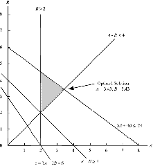
20. a.
| Max | 3A | + | 2B | ||||||
| s.t. | |||||||||
| A | + | B | - S1 | = | 4 | ||||
| 3A | + | 4B | + S2 | = | 24 | ||||
| A | - S3 | = | 2 | ||||||
| A | - | B | - S4 | = | 0 |
A, B, S1, S2, S3, S4 ³ 0
b.
c. S1 = (3.43 + 3.43) - 4 = 2.86
S2 = 24 - [3(3.43) + 4(3.43)] = 0
S3 = 3.43 - 2 = 1.43
S4 = 0 - (3.43 - 3.43) = 0
21. a. and b.
c. Optimal solution occurs at the intersection of constraints 1 and 2. For constraint 2,
B = 10 + A
Substituting for B in constraint 1 we obtain
| 5A + 5(10 + A) | = 400 |
| 5A + 50 + 5A | = 400 |
| 10A | = 350 |
| A | = 35 |
B = 10 + A = 10 + 35 = 45
Optimal solution is A = 35, B = 45
d. Because the optimal solution occurs at the intersection of constraints 1 and 2, these are binding constraints.
e. Constraint 3 is the nonbinding constraint. At the optimal solution 1A + 3B = 1(35) + 3(45) = 170. Because 170 exceeds the right-hand side value of 90 by 80 units, there is a surplus of 80 associated with this constraint.
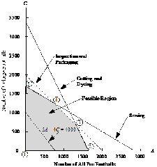
22. a.
b.
| Extreme Point | Coordinates | Profit |
| 1 | (0, 0) | 5(0) + 4(0) = 0 |
| 2 | (1700, 0) | 5(1700) + 4(0) = 8500 |
| 3 | (1400, 600) | 5(1400) + 4(600) = 9400 |
| 4 | (800, 1200) | 5(800) + 4(1200) = 8800 |
| 5 | (0, 1680) | 5(0) + 4(1680) = 6720 |
Extreme point 3 generates the highest profit.
c. Optimal solution is A = 1400, C = 600
d. The optimal solution occurs at the intersection of the cutting and dyeing constraint and the inspection and packaging constraint. Therefore these two constraints are the binding constraints.
e. New optimal solution is A = 800, C = 1200
Profit = 4(800) + 5(1200) = 9200
23. a. Let E = number of units of the EZ-Rider produced
L = number of units of the Lady-Sport produced
| Max | 2400E | + | 1800L | |||
| s.t. | ||||||
| 6E | + | 3L | £ | 2100 | Engine time | |
| L | £ | 280 | Lady-Sport maximum | |||
| 2E | + | 2.5L | £ | 1000 | Assembly and testing |
E, L ³ 0
 |
b.
c. The binding constraints are the manufacturing time and the assembly and testing time.
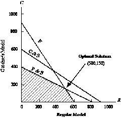
24. a. Let R = number of units of regular model.
C = number of units of catcher’s model.
| Max | 5R | + | 8C | ||
| s.t. | |||||
| 1R | + | 3/2 C | £ | 900 Cutting and sewing | |
| 1/2 R | + | 1/3 C | £ | 300 Finishing | |
| 1/8 R | + | 1/4 C | £ | 100 Packing and Shipping |
R, C ³ 0
b.
c. 5(500) + 8(150) = $3,700
d. C & S 1(500) + 3/2(150) = 725
F 1/2(500) + 1/3(150) = 300
P & S 1/8(500) + 1/4(150) = 100
e.
| Department | Capacity | Usage | Slack |
| C & S | 900 | 725 | 175 hours |
| F | 300 | 300 | 0 hours |
| P & S | 100 | 100 | 0 hours |
25. a. Let B = percentage of funds invested in the bond fund
S = percentage of funds invested in the stock fund
| Max | 0.06 B | + | 0.10 S | |||
| s.t. | ||||||
| B | ³ | 0.3 | Bond fund minimum | |||
| 0.06 B | + | 0.10 S | ³ | 0.075 | Minimum return | |
| B | + | S | = | 1 | Percentage requirement |
b. Optimal solution: B = 0.3, S = 0.7
Value of optimal solution is 0.088 or 8.8%
26. a. a. Let N = amount spent on newspaper advertising
R = amount spent on radio advertising
| Max | 50N | + | 80R | |||||
| s.t. | ||||||||
| N | + | R | = | 1000 | Budget | |||
| N | ³ | 250 | Newspaper min. | |||||
| R | ³ | 250 | Radio min. | |||||
| N | -2R | ³ | 0 | News ³ 2 Radio | ||||
N, R ³ 0
b.
27. Let I = Internet fund investment in thousands
B = Blue Chip fund investment in thousands
| Max | 0.12I | + | 0.09B | |||
| s.t. | ||||||
| 1I | + | 1B | £ | 50 | Available investment funds | |
| 1I | £ | 35 | Maximum investment in the internet fund | |||
| 6I | + | 4B | £ | 240 | Maximum risk for a moderate investor |
I, B ³ 0
 |
Internet fund $20,000
Blue Chip fund $30,000
Annual return $ 5,100
b. The third constraint for the aggressive investor becomes
6I + 4B £ 320
This constraint is redundant; the available funds and the maximum Internet fund investment constraints define the feasible region. The optimal solution is:
Internet fund $35,000
Blue Chip fund $15,000
Annual return $ 5,550
The aggressive investor places as much funds as possible in the high return but high risk Internet fund.
c. The third constraint for the conservative investor becomes
6I + 4B £ 160
This constraint becomes a binding constraint. The optimal solution is
Internet fund $0
Blue Chip fund $40,000
Annual return $ 3,600
The slack for constraint 1 is $10,000. This indicates that investing all $50,000 in the Blue Chip fund is still too risky for the conservative investor. $40,000 can be invested in the Blue Chip fund. The remaining $10,000 could be invested in low-risk bonds or certificates of deposit.
28. a. Let W = number of jars of Western Foods Salsa produced
M = number of jars of Mexico City Salsa produced
| Max | 1W | + | 1.25M | |||
| s.t. | ||||||
| 5W | 7M | £ | 4480 | Whole tomatoes | ||
| 3W | + | 1M | £ | 2080 | Tomato sauce | |
| 2W | + | 2M | £ | 1600 | Tomato paste |
W, M ³ 0
Note: units for constraints are ounces
b. Optimal solution: W = 560, M = 240
Value of optimal solution is 860
29. a. Let B = proportion of Buffalo's time used to produce component 1
D = proportion of Dayton's time used to produce component 1
| Maximum Daily Production | ||
| Component 1 | Component 2 | |
| Buffalo | 2000 | 1000 |
| Dayton | 600 | 1400 |
Number of units of component 1 produced: 2000B + 600D
Number of units of component 2 produced: 1000(1 - B) + 600(1 - D)
For assembly of the ignition systems, the number of units of component 1 produced must equal the number of units of component 2 produced.
Therefore,
2000B + 600D = 1000(1 - B) + 1400(1 - D)
2000B + 600D = 1000 - 1000B + 1400 - 1400D
3000B + 2000D = 2400
Note: Because every ignition system uses 1 unit of component 1 and 1 unit of component 2, we can maximize the number of electronic ignition systems produced by maximizing the number of units of subassembly 1 produced.
Max 2000B + 600D
In addition, B £ 1 and D £ 1.
The linear programming model is:
| Max | 2000B | + 600D | |
| s.t. | |||
| 3000B | + 2000D | = 2400 | |
| B | £ 1 | ||
| D | £ 1 | ||
| B, D | ³ 0 | ||
| |
The graphical solution is shown below.
 |
Optimal Solution: B = .8, D = 0
Optimal Production Plan
Buffalo - Component 1 .8(2000) = 1600
Buffalo - Component 2 .2(1000) = 200
Dayton - Component 1 0(600) = 0
Dayton - Component 2 1(1400) = 1400
Total units of electronic ignition system = 1600 per day.
30. a. Let E = number of shares of Eastern Cable
C = number of shares of ComSwitch
| Max | 15E | + | 18C | |||
| s.t. | ||||||
| 40E | + | 25C | £ | 50,000 | Maximum Investment | |
| 40E | ³ | 15,000 | Eastern Cable Minimum | |||
| 25C | ³ | 10,000 | ComSwitch Minimum | |||
| 25C | £ | 25,000 | ComSwitch Maximum |
E, C ³ 0
 |
b.
c. There are four extreme points: (375,400); (1000,400);(625,1000); (375,1000)
d. Optimal solution is E = 625, C = 1000
Total return = $27,375
31.
Objective Function Value = 13
32.
|
|
|
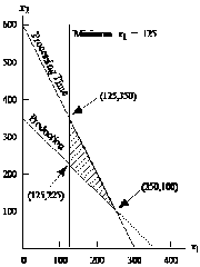
| Extreme Points | Objective Function Value | Surplus Demand | Surplus Total Production | Slack Processing Time |
| (A = 250, B = 100) | 800 | 125 | — | — |
| (A = 125, B = 225) | 925 | — | — | 125 |
| (A = 125, B = 350) | 1300 | — | 125 | — |
33. a.
|
|
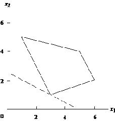
Optimal Solution: A = 3, B = 1, value = 5
b.
| (1) | 3 + 4(1) = 7 | Slack = 21 - 7 = 14 |
| (2) | 2(3) + 1 = 7 | Surplus = 7 - 7 = 0 |
| (3) | 3(3) + 1.5 = 10.5 | Slack = 21 - 10.5 = 10.5 |
| (4) | -2(3) +6(1) = 0 | Surplus = 0 - 0 = 0 |
c.
|
|

Optimal Solution: A = 6, B = 2, value = 34
34. a.
|
|

b. There are two extreme points: (A = 4, B = 1) and (A = 21/4, B = 9/4)
c. The optimal solution is A = 4, B = 1
35. a.
| Min | 6A | + | 4B | + | 0S1 | + | 0S2 | + | 0S3 | ||
| s.t. | |||||||||||
| 2A | + | 1B | - | S1 | = | 12 | |||||
| 1A | + | 1B | - | S2 | = | 10 | |||||
| 1B | + | S3 | = | 4 |
A, B, S1, S2, S3 ³ 0
b. The optimal solution is A = 6, B = 4.
c. S1 = 4, S2 = 0, S3 = 0.
36. a. Let T = number of training programs on teaming
P = number of training programs on problem solving
| Max | 10,000T | + | 8,000P | |||
| s.t. | ||||||
| T | ³ | 8 | Minimum Teaming | |||
| P | ³ | 10 | Minimum Problem Solving | |||
| T | + | P | ³ | 25 | Minimum Total | |
| 3 T | + | 2 P | £ | 84 | Days Available |
T, P ³ 0
b.
 |
c. There are four extreme points: (15,10); (21.33,10); (8,30); (8,17)
d. The minimum cost solution is T = 8, P = 17
Total cost = $216,000
37.
| Regular | Zesty | ||
| Mild | 80% | 60% | 8100 |
| Extra Sharp | 20% | 40% | 3000 |
Let R = number of containers of Regular
Z = number of containers of Zesty
Each container holds 12/16 or 0.75 pounds of cheese
Pounds of mild cheese used = 0.80 (0.75) R + 0.60 (0.75) Z
= 0.60 R + 0.45 Z
Pounds of extra sharp cheese used = 0.20 (0.75) R + 0.40 (0.75) Z
= 0.15 R + 0.30 Z
Cost of Cheese = Cost of mild + Cost of extra sharp
= 1.20 (0.60 R + 0.45 Z) + 1.40 (0.15 R + 0.30 Z)
= 0.72 R + 0.54 Z + 0.21 R + 0.42 Z
= 0.93 R + 0.96 Z
Packaging Cost = 0.20 R + 0.20 Z
Total Cost = (0.93 R + 0.96 Z) + (0.20 R + 0.20 Z)
= 1.13 R + 1.16 Z
Revenue = 1.95 R + 2.20 Z
Profit Contribution = Revenue - Total Cost
= (1.95 R + 2.20 Z) - (1.13 R + 1.16 Z)
= 0.82 R + 1.04 Z
| Max | 0.82 R | + | 1.04 Z | |||
| s.t. | ||||||
| 0.60 R | + | 0.45 Z | £ | 8100 | Mild | |
| 0.15 R | + | 0.30 Z | £ | 3000 | Extra Sharp |
R, Z ³ 0
Optimal Solution: R = 9600, Z = 5200, profit = 0.82(9600) + 1.04(5200) = $13,280
38. a. Let S = yards of the standard grade material per frame
P = yards of the professional grade material per frame
| Min | 7.50S | + | 9.00P | |||
| s.t. | ||||||
| 0.10S | + | 0.30P | ³ | 6 | carbon fiber (at least 20% of 30 yards) | |
| 0.06S | + | 0.12P | £ | 3 | kevlar (no more than 10% of 30 yards) | |
| S | + | P | = | 30 | total (30 yards) |
S, P ³ 0
 |
b.
c.
| Extreme Point | Cost |
| (15, 15) | 7.50(15) + 9.00(15) = 247.50 |
| (10, 20) | 7.50(10) + 9.00(20) = 255.00 |
The optimal solution is S = 15, P = 15
d. Optimal solution does not change: S = 15 and P = 15. However, the value of the optimal solution is reduced to 7.50(15) + 8(15) = $232.50.
e. At $7.40 per yard, the optimal solution is S = 10, P = 20. The value of the optimal solution is reduced to 7.50(10) + 7.40(20) = $223.00. A lower price for the professional grade will not change the S = 10, P = 20 solution because of the requirement for the maximum percentage of kevlar (10%).
39. a. Let S = number of units purchased in the stock fund
M = number of units purchased in the money market fund
| Min | 8S | + | 3M | ||
| s.t. | |||||
| 50S | + | 100M | £ | 1,200,000 Funds available | |
| 5S | + | 4M | ³ | 60,000 Annual income | |
| M | ³ | 3,000 Minimum units in money market |
S, M, ³ 0
|
|
|

Optimal Solution: S = 4000, M = 10000, value = 62000
b. Annual income = 5(4000) + 4(10000) = 60,000
c. Invest everything in the stock fund.
40. Let P1 = gallons of product 1
P2 = gallons of product 2
| Min | 1P1 | + | 1P2 | ||
| s.t. | |||||
| 1P1 | + | ³ | 30 Product 1 minimum | ||
| 1P2 | ³ | 20 Product 2 minimum | |||
| 1P1 | + | 2P2 | ³ | 80 Raw material |
P1, P2 ³ 0
 |
Optimal Solution: P1 = 30, P2 = 25 Cost = $55
41. a. Let R = number of gallons of regular gasoline produced
P = number of gallons of premium gasoline produced
| Max | 0.30R | + | 0.50P | |||
| s.t. | ||||||
| 0.30R | + | 0.60P | £ | 18,000 | Grade A crude oil available | |
| 1R | + | 1P | £ | 50,000 | Production capacity | |
| 1P | £ | 20,000 | Demand for premium |
R, P ³ 0
 |
b.
Optimal Solution:
40,000 gallons of regular gasoline
10,000 gallons of premium gasoline
Total profit contribution = $17,000
c.
| Constraint | Value of Slack Variable | Interpretation |
| 1 | 0 | All available grade A crude oil is used |
| 2 | 0 | Total production capacity is used |
| 3 | 10,000 | Premium gasoline production is 10,000 gallons less than the maximum demand |
d. Grade A crude oil and production capacity are the binding constraints.
|
42.
|
|

43.
|
|

44. a.
|
|

b. New optimal solution is A = 0, B = 3, value = 6.
45. a.
|
|
|
|
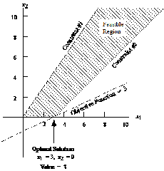
b. Feasible region is unbounded.
c. Optimal Solution: A = 3, B = 0, z = 3.
d. An unbounded feasible region does not imply the problem is unbounded. This will only be the case when it is unbounded in the direction of improvement for the objective function.
46. Let N = number of sq. ft. for national brands
G = number of sq. ft. for generic brands
Problem Constraints:
| N | + | G | £ | 200 | Space available | |
| N | ³ | 120 | National brands | |||
| G | ³ | 20 | Generic |
| Extreme Point | N | G |
| 1 | 120 | 20 |
| 2 | 180 | 20 |
| 3 | 120 | 80 |
a. Optimal solution is extreme point 2; 180 sq. ft. for the national brand and 20 sq. ft. for the generic brand.
b. Alternative optimal solutions. Any point on the line segment joining extreme point 2 and extreme point 3 is optimal.
c. Optimal solution is extreme point 3; 120 sq. ft. for the national brand and 80 sq. ft. for the generic brand.
|
|

Alternative optimal solutions exist at extreme points (A = 125, B = 225) and (A = 250, B = 100).
Cost = 3(125) + 3(225) = 1050
or
Cost = 3(250) + 3(100) = 1050
The solution (A = 250, B = 100) uses all available processing time. However, the solution
(A = 125, B = 225) uses only 2(125) + 1(225) = 475 hours.
Thus, (A = 125, B = 225) provides 600 - 475 = 125 hours of slack processing time which may be used for other products.
48.
Possible Actions:
i. Reduce total production to A = 125, B = 350 on 475 gallons.
ii. Make solution A = 125, B = 375 which would require 2(125) + 1(375) = 625 hours of processing time. This would involve 25 hours of overtime or extra processing time.
iii. Reduce minimum A production to 100, making A = 100, B = 400 the desired solution.
49. a. Let P = number of full-time equivalent pharmacists
T = number of full-time equivalent physicians
The model and the optimal solution are shown below:
MIN 40P+10T
S.T.
1) P+T >=250
2) 2P-T>=0
3) P>=90
| Optimal Objective Value | ||
| 5200.00000 | ||
| Variable | Value | Reduced Cost |
| P | 90.00000 | 0.00000 |
| T | 160.00000 | 0.00000 |
| Constraint | Slack/Surplus | Dual Value |
| 1 | 0.00000 | 10.00000 |
| 2 | 20.00000 | 0.00000 |
| 3 | 0.00000 | 30.00000 |
The optimal solution requires 90 full-time equivalent pharmacists and 160 full-time equivalent technicians. The total cost is $5200 per hour.
b.
| Current Levels | Attrition | Optimal Values | New Hires Required | |
| Pharmacists | 85 | 10 | 90 | 15 |
| Technicians | 175 | 30 | 160 | 15 |
The payroll cost using the current levels of 85 pharmacists and 175 technicians is 40(85) + 10(175) = $5150 per hour.
The payroll cost using the optimal solution in part (a) is $5200 per hour.
Thus, the payroll cost will go up by $50
50. Let M = number of Mount Everest Parkas
R = number of Rocky Mountain Parkas
| Max | 100M | + | 150R | ||
| s.t. | |||||
| 30M | + | 20R | £ | 7200 Cutting time | |
| 45M | + | 15R | £ | 7200 Sewing time | |
| 0.8M | - | 0.2R | ³ | 0 % requirement |
Note: Students often have difficulty formulating constraints such as the % requirement constraint. We encourage our students to proceed in a systematic step-by-step fashion when formulating these types of constraints. For example:
M must be at least 20% of total production
M ³ 0.2 (total production)
M ³ 0.2 (M + R)
M ³ 0.2M + 0.2R
0.8M - 0.2R ³ 0
The optimal solution is M = 65.45 and R = 261.82; the value of this solution is z = 100(65.45) + 150(261.82) = $45,818. If we think of this situation as an on-going continuous production process, the fractional values simply represent partially completed products. If this is not the case, we can approximate the optimal solution by rounding down; this yields the solution M = 65 and R = 261 with a corresponding profit of $45,650.
51. Let C = number sent to current customers
N = number sent to new customers
Note:
Number of current customers that test drive = .25 C
Number of new customers that test drive = .20 N
Number sold = .12 ( .25 C ) + .20 (.20 N )
= .03 C + .04 N
| Max | .03C | + | .04N | |||
| s.t. | ||||||
| .25 C | ³ | 30,000 | Current Min | |||
| .20 N | ³ | 10,000 | New Min | |||
| .25 C | - | .40 N | ³ | 0 | Current vs. New | |
| 4 C | + | 6 N | £ | 1,200,000 | Budget |
C, N, ³ 0
 |
52. Let S = number of standard size rackets
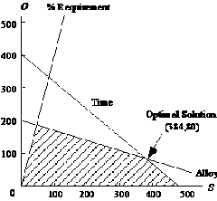
O = number of oversize size rackets
| Max | 10S | + | 15O | |||
| s.t. | ||||||
| 0.8S | - | 0.2O | ³ | 0 | % standard | |
| 10S | + | 12O | £ | 4800 | Time | |
| 0.125S | + | 0.4O | £ | 80 | Alloy |
S, O, ³ 0
53. a. Let R = time allocated to regular customer service
N = time allocated to new customer service
| Max | 1.2R | + | N | ||
| s.t. | |||||
| R | + | N | £ | 80 | |
| 25R | + | 8N | ³ | 800 | |
| -0.6R | + | N | ³ | 0 |
R, N, ³ 0
b.
| Optimal Objective Value | ||
| 90.00000 | ||
| Variable | Value | Reduced Cost |
| R | 50.00000 | 0.00000 |
| N | 30.00000 | 0.00000 |
| Constraint | Slack/Surplus | Dual Value |
| 1 | 0.00000 | 1.12500 |
| 2 | 690.00000 | 0.00000 |
| 3 | 0.00000 | -0.12500 |
Optimal solution: R = 50, N = 30, value = 90
HTS should allocate 50 hours to service for regular customers and 30 hours to calling on new customers.
54. a. Let M1 = number of hours spent on the M-100 machine
M2 = number of hours spent on the M-200 machine
Total Cost
6(40)M1 + 6(50)M2 + 50M1 + 75M2 = 290M1 + 375M2
Total Revenue
25(18)M1 + 40(18)M2 = 450M1 + 720M2
Profit Contribution
(450 - 290)M1 + (720 - 375)M2 = 160M1 + 345M2
| Max | 160 M1 | + | 345M2 | |||
| s.t. | ||||||
| M1 | £ | 15 | M-100 maximum | |||
| M2 | £ | 10 | M-200 maximum | |||
| M1 | ³ | 5 | M-100 minimum | |||
| M2 | ³ | 5 | M-200 minimum | |||
| 40 M1 | + | 50 M2 | £ | 1000 | Raw material available |
M1, M2 ³ 0
b.
| Optimal Objective Value | ||
| 5450.00000 | ||
| Variable | Value | Reduced Cost |
| M1 | 12.50000 | 0.00000 |
| M2 | 10.00000 | 145.00000 |
| Constraint | Slack/Surplus | Dual Value |
| 1 | 2.50000 | 0.00000 |
| 2 | 0.00000 | 145.00000 |
| 3 | 7.50000 | 0.00000 |
| 4 | 5.00000 | 0.00000 |
| 5 | 0.00000 | 4.00000 |
The optimal decision is to schedule 12.5 hours on the M-100 and 10 hours on the M-200.
55. Mr. Krtick’s solution cannot be optimal. Every department has unused hours, so there are no binding constraints. With unused hours in every department, clearly some more product can be made.
56. No, it is not possible that the problem is now infeasible. Note that the original problem was feasible (it had an optimal solution). Every solution that was feasible is still feasible when we change the constraint to less-than-or-equal-to, since the new constraint is satisfied at equality (as well as inequality). In summary, we have relaxed the constraint so that the previous solutions are feasible (and possibly more satisfying the constraint as strict inequality).
57. Yes, it is possible that the modified problem is infeasible. To see this, consider a redundant greater-than-or-equal to constraint as shown below. Constraints 2, 3, and 4 form the feasible region and constraint 1 is redundant. Change constraint 1 to less-than-or-equal-to and the modified problem is infeasible.
Original Problem:
Modified Problem:
58. It makes no sense to add this constraint. The objective of the problem is to minimize the number of products needed so that everyone’s top three choices are included. There are only two possible outcomes relative to the boss’ new constraint. First, suppose the minimum number of products is <= 15, then there was no need for the new constraint. Second, suppose the minimum number is > 15. Then the new constraint makes the problem infeasible.
Chapter 2—An Introduction to Linear Programming
MULTIPLE CHOICE
1. The maximization or minimization of a quantity is the
| a. | goal of management science. |
| b. | decision for decision analysis. |
| c. | constraint of operations research. |
| d. | objective of linear programming. |
ANS: D PTS: 1 TOP: Introduction
2. Decision variables
| a. | tell how much or how many of something to produce, invest, purchase, hire, etc. |
| b. | represent the values of the constraints. |
| c. | measure the objective function. |
| d. | must exist for each constraint. |
ANS: A PTS: 1 TOP: Objective function
3. Which of the following is a valid objective function for a linear programming problem?
| a. | Max 5xy |
| b. | Min 4x + 3y + (2/3)z |
| c. | Max 5x2 + 6y2 |
| d. | Min (x1 + x2)/x3 |
ANS: B PTS: 1 TOP: Objective function
4. Which of the following statements is NOT true?
| a. | A feasible solution satisfies all constraints. |
| b. | An optimal solution satisfies all constraints. |
| c. | An infeasible solution violates all constraints. |
| d. | A feasible solution point does not have to lie on the boundary of the feasible region. |
ANS: C PTS: 1 TOP: Graphical solution
5. A solution that satisfies all the constraints of a linear programming problem except the nonnegativity constraints is called
| a. | optimal. |
| b. | feasible. |
| c. | infeasible. |
| d. | semi-feasible. |
ANS: C PTS: 1 TOP: Graphical solution
6. Slack
| a. | is the difference between the left and right sides of a constraint. |
| b. | is the amount by which the left side of a £ constraint is smaller than the right side. |
| c. | is the amount by which the left side of a ³ constraint is larger than the right side. |
| d. | exists for each variable in a linear programming problem. |
ANS: B PTS: 1 TOP: Slack variables
7. To find the optimal solution to a linear programming problem using the graphical method
| a. | find the feasible point that is the farthest away from the origin. |
| b. | find the feasible point that is at the highest location. |
| c. | find the feasible point that is closest to the origin. |
| d. | None of the alternatives is correct. |
ANS: D PTS: 1 TOP: Extreme points
8. Which of the following special cases does not require reformulation of the problem in order to obtain a solution?
| a. | alternate optimality |
| b. | infeasibility |
| c. | unboundedness |
| d. | each case requires a reformulation. |
ANS: A PTS: 1 TOP: Special cases
9. The improvement in the value of the objective function per unit increase in a right-hand side is the
| a. | sensitivity value. |
| b. | dual price. |
| c. | constraint coefficient. |
| d. | slack value. |
ANS: B PTS: 1 TOP: Right-hand sides
10. As long as the slope of the objective function stays between the slopes of the binding constraints
| a. | the value of the objective function won't change. |
| b. | there will be alternative optimal solutions. |
| c. | the values of the dual variables won't change. |
| d. | there will be no slack in the solution. |
ANS: C PTS: 1 TOP: Objective function
11. Infeasibility means that the number of solutions to the linear programming models that satisfies all constraints is
| a. | at least 1. |
| b. | 0. |
| c. | an infinite number. |
| d. | at least 2. |
ANS: B PTS: 1 TOP: Alternate optimal solutions









No comments:
Post a Comment